Pexp and qexp Tutorial
Motivation for Exponential Functions
The Exponential distribution is used to model events that occur randomly and independently at a constant rate, such as customer arrivals. It is tailored for positive random variables often interpreted as the wait time for a specific event. This family of distributions is defined by a single parameter, typically representing either the mean wait time (β > 0) or its reciprocal, the average rate (λ > 0) at which an event happens.
The Probability Density Function (PDF) of the exponential distribution illustrates the probability distribution of a continuous random variable, whereas the Cumulative Distribution Function (CDF), obtained through the integral of the PDF, conveys the probability that a random variable is equal to or less than a specified value.
The functions pexp and qexp calculate the cumulative probability for a specified quantile and vice versa. Additionally, these functions allow you to plot both the PDF and CDF, providing a visual representation of the cumulative probability associated with a particular quantile. The CDF graph plots the cumulative probability against the specific quantile, while the PDF graph illustrates the cumulative probability up to that quantile through the area under the curve.
Usage of pexp and qexp
In this section, we demonstrate the usage of pexp and qexp for addressing statistical questions concerning the exponential distribution. The dataset utilized in this tutorial is the lung dataset from the survival package in R, a comprehensive and widely utilized package for survival analysis. The package is publicly available and distributed under LGPL-2, LGPL-2.1, or LGPL-3 licenses, making it a popular resource in statistical analyses and academic research. For the purpose of this tutorial, we have exported the lung dataset from the survival package and saved it as a CSV file in the docs/data/ directory to ensure ease of access and transparency in data usage.
Specifically, the lung dataset includes data on the survival of patients with advanced lung cancer, featuring variables such as survival time, patient status, age, sex, and various clinical measures. This dataset’s rich, real-world context makes it a go-to choice for demonstrating survival analysis techniques. In this tutorial, we will delve into the dataset, specifically focusing on the time variable, which typically represents the survival time of the patients.
import pandas as pd
import matplotlib.pyplot as plt

# Load the dataset
file_path = "../docs/data/lung_dataset.csv"
lung_df = pd.read_csv(file_path)
lung_df.head()
| inst | time | status | age | sex | ph.ecog | ph.karno | pat.karno | meal.cal | wt.loss | |
|---|---|---|---|---|---|---|---|---|---|---|
| 0 | 3.0 | 306 | 2 | 74 | 1 | 1.0 | 90.0 | 100.0 | 1175.0 | NaN |
| 1 | 3.0 | 455 | 2 | 68 | 1 | 0.0 | 90.0 | 90.0 | 1225.0 | 15.0 |
| 2 | 3.0 | 1010 | 1 | 56 | 1 | 0.0 | 90.0 | 90.0 | NaN | 15.0 |
| 3 | 5.0 | 210 | 2 | 57 | 1 | 1.0 | 90.0 | 60.0 | 1150.0 | 11.0 |
| 4 | 1.0 | 883 | 2 | 60 | 1 | 0.0 | 100.0 | 90.0 | NaN | 0.0 |
Let’s assume we want to answer two questions:
What is the cumulative probability of survival up to the median survival time?
What is the survival time above which only the top 5% of patients survive?
First, let’s look at the distribution of survival times. We can visualize this with a histogram and determine if it closely resembles an exponential distribution.
# Visualize the distribution of survival times
plt.hist(lung_df['time'], bins=20, color='lightblue', edgecolor='black')
plt.title("Distribution of Patients' Survival Time")
plt.xlabel('Survival Time')
plt.ylabel('Frequency')
plt.show()
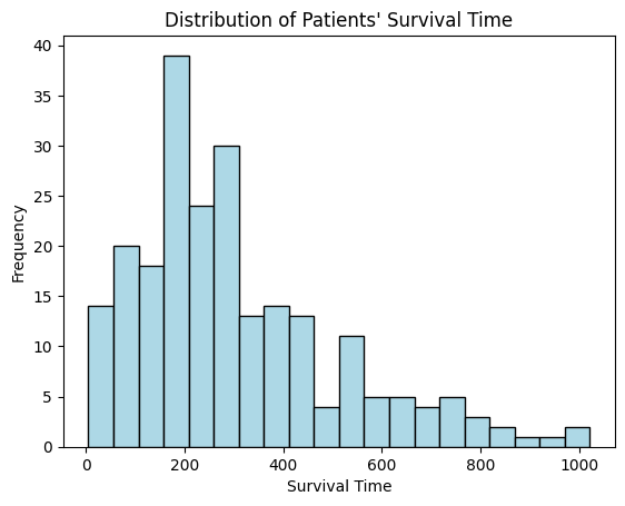
From the plot above, we could see the distribution closely resemble an exponential pattern, making it suitable for analysis using our pexp and qexp functions to address our statistical inquiries.
from mathdistops import pexp, qexp
# Calculate the rate as the reciprocal of the mean time
rate = 1 / lung_df['time'].mean()

# Calculate the cumulative probability up to the median survival time
q = lung_df['time'].median()
df, fig = pexp(q, rate, graph=True)
df
| Quantile | Cumulative probability | |
|---|---|---|
| 0 | 255.5 | 0.567021 |
Let’s analyze the results and address the first question.
Question: What is the cumulative probability of survival up to the median survival time?
Answer: Based on the output from the pexp function, we find that the cumulative probability of survival up to the median survival time (255.5 days) is approximately 0.567 or 56.7%. This indicates that about 56.7% of patients in this dataset are expected to survive up to 255.5 days.
(Note: we would anticipate the cumulative probability of the median to e 0.5. However, it’s important to remember that the exponential distribution doesn’t perfectly describe the data; it merely serves as an approximation. This explains why we observe a value of 0.567 instead of 0.5.)
fig
In the output charts, the Probability Density Function (PDF) presents the distribution of survival times. The shaded area under the curve shows the cumulative probability of the median survival time of 255.5 days. On the Cumulative Distribution Function (CDF), the same vertical line intersects the curve, denoting that approximately 56.7% of patients are expected to survive up to this point. This visual distinction in the charts, with the shaded area under the PDF curve and the corresponding point on the CDF, provides a clear and intuitive understanding of the distribution of survival times and the cumulative probability up to the median survival time.
Now, let’s address the second question by using the qexp function to find the survival time above which only the top 5% of patients are expected to survive.
# Find the survival time corresponding to the top 5 percentile
df, fig = qexp(0.95, rate=rate, graph=True)
df
| Probability | Quantile | |
|---|---|---|
| 0 | 0.95 | 914.39472 |
The output from the qexp function reveals the quantile value for the top 5% of patients, setting a survival time benchmark above which patients are considered to be among the longest survivors.
Question: What is the threshold of survival time that marks the longest surviving top 5% of patients?
Answer: The calculated quantile value from the qexp function indicates that patients surviving beyond 914.39472 days are within the top 5% in terms of survival time.
fig
In the chart from the qexp function, the top 5% survival time threshold is visualized as a horizontal dotted line at 914.39472 days on the CDF chart. The point where this line meets the cumulative distribution curve emphasizes that only 5% of patients survive longer than this time. In the PDF the 95% percentile corresponds to the blue shaded area under the PDF.
Through this tutorial, we’ve navigated the practical applications of the pexp and qexp functions from our Python package, gaining both numerical insights and visual interpretations. We hope this tutorial serves as a valuable guide in your data analysis efforts, enabling you to use these functions to discover important patterns and make informed decisions in your work.